Variational Autoencoder
Variational Autoencoders (VAEs) are a class of generative models that are widely used in machine learning for their ability to learn efficient latent representations of data. They extend traditional/vanilla autoencoders by imposing a probabilistic structure on the latent space, making them capable of generating new data samples.
The key idea behind VAEs is to map high-dimensional input data to a lower-dimensional latent space, from which new data points can be sampled and decoded back to the original input space.
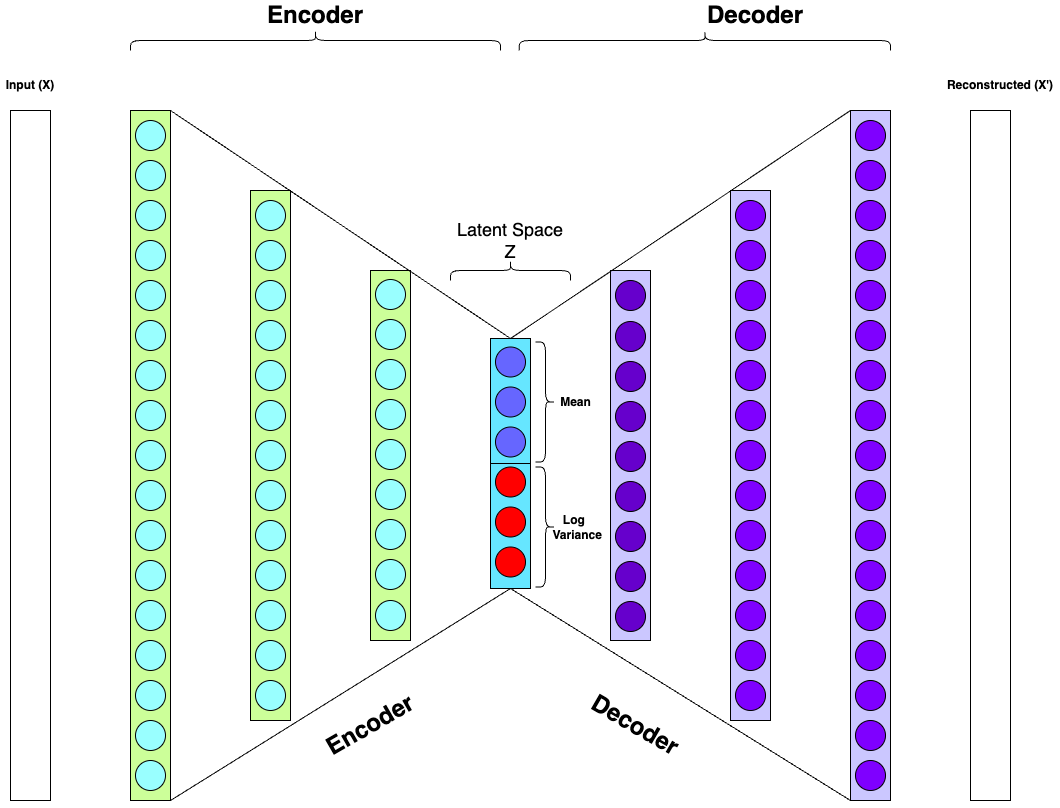
Figure (i) by KB designed using draw.io
Figure (ii) by KB designed using gifski. You will find this interactive model at the bottom of this page.
The VAE Architecture
A VAE consists of two main components: the encoder and the decoder.
- Encoder: Maps the input data to a latent space by outputting two vectors: the mean (μ) and the log-variance (log(σ²)) of the latent distribution.
- Decoder: Uses a sampled latent vector to reconstruct the original data from the lower-dimensional latent space.
These two components are trained simultaneously to minimize the reconstruction error and the Kullback-Leibler (KL) divergence between the learned latent distribution and a prior distribution (typically a standard Gaussian).
The goal of a VAE is to learn a distribution \(p(x)\) that best approximates the data \(x\) by sampling latent variables \(z\) from a learned distribution \(q(z|x)\) and using these to reconstruct the data \(x\).
Reparameterization Trick
In Variational Autoencoders (VAEs), the encoder network maps an input \(x\) to a distribution over the latent space. This distribution is typically Gaussian with a mean \(\mu\) and a variance \(\sigma^2\). To generate the latent variable \(z\), we would ideally sample it from this distribution. The problem arises, however, with the sampling process itself. Sampling introduces stochasticity (randomness), which disrupts the backpropagation process needed for training the model.
The core challenge is that backpropagation requires a differentiable function, i.e a full deterministic computational graph. However, the operation of drawing a random sample from the Gaussian distribution is not deterministic. This is a significant issue for training the encoder network, as backpropagation would fail without a method to handle this stochastic step.
The reparameterization trick is a technique that addresses this problem by re-expressing the sampling process in a way that allows gradients to propagate through it. Instead of directly sampling \(z\) from the Gaussian distribution, we reparameterize the latent variable \(z\) as a deterministic function of \(\mu\), \(\sigma\), and a random noise term \(\epsilon\) drawn from a standard normal distribution \( \mathcal{N}(0, 1)\). Specifically, the reparameterization is expressed as:
Here, \(\mu\) and \(\sigma\) are the mean and standard deviation of the latent distribution, which are both outputs of the encoder network. The term \(\epsilon\) represents random noise drawn from a standard normal distribution, which introduces the randomness into the latent variable. This formulation has a key advantage: \(z\) is now expressed as a deterministic function of \(\mu\), \(\sigma\), and \(\epsilon\), where the randomness is isolated in \(\epsilon\), which does not depend on the network parameters. This means that the values of \(\mu\) and \(\sigma\) are directly controlled by the network, and gradients can be backpropagated through them during training.
Intuition
To understand this intuitively, consider that \(\mu\) and \(\sigma\) control the location (mean) and spread (variance) of the latent distribution. I will show what this means with an actual coding implementation as well as a visualization of the latent space in 3D. Think of the reparameterization trick as "shifting and scaling" the randomness (\(\epsilon\)):
- \(\mu\) shifts the distribution.
- \(\sigma\) scales the distribution.
The reparameterization trick allows the model to preserve the stochasticity of the latent variable while ensuring that the process remains differentiable and trainable via backpropagation.
ELBO (Evidence Lower Bound):
A Variational Autoencoder (VAE) learns a probabilistic mapping from a high-dimensional data space \( x \) to a lower-dimensional latent space \( z \). The objective of the VAE is to maximize the likelihood of the data, but instead of directly maximizing \( p(x) \), we maximize the Evidence Lower Bound (ELBO) due to the intractability of the marginal likelihood.
The VAE maximizes the ELBO, which is a lower bound on the log-likelihood of the data:
Where:
- \( p(x) \) is the marginal likelihood (the probability of the data).
- \( q(z|x) \) is the approximate posterior distribution of the latent variable \( z \) given the input \( x \).
- \( p(x|z) \) is the likelihood of the data given the latent variable \( z \) (the decoder network).
- \( p(z) \) is the prior distribution over the latent variable \( z \), often chosen as a standard normal \( \mathcal{N}(0, I) \).
- The second term is the **KL divergence** which penalizes the divergence between the learned posterior and the prior.
KL Divergence:
The KL divergence between the approximate posterior \( q(z|x) \) and the prior \( p(z) \) is computed as:
Where:
- \( \mu \) and \( \sigma^2 \) are the mean and variance of the approximate posterior distribution \( q(z|x) = \mathcal{N}(\mu(x), \sigma^2(x)) \).
- \( p(z) = \mathcal{N}(0, I) \) is the standard normal prior over \( z \).
VAE Loss Function:
The total loss function for the VAE combines the reconstruction loss and the KL divergence term:
The reconstruction loss ensures that the decoder can generate accurate data samples from the latent variable, while the KL divergence ensures that the learned latent distribution is close to the prior, helping with regularization.
An Implementation: That is enough intro, now where is the real code you say?
I have included the actual source code (github link) of this implementation of a variational autoencoder here: https://github.com/KrishnaMBhattarai/VariationalAutoencoder
Well, that is kind of boring. Even better is if you want to run and tweak the model in real time, I have also included a link to google colab, so you can open the notebook with Google Colab directly: https://colab.research.google.com/github/KrishnaMBhattarai/VariationalAutoencoder/blob/main/VariationalAutoencoder.ipynb
Now, what I hope someone will find useful is that, I have spent the time to describe every line of the architecture in the code with descriptive comments. This will help a student or researcher really understand how the mathematics above gets implemented in action. If you dont want to click on the links above, let's look at the code here:
First the architectural setup of the model. Now this will look normal to a student who has studied neural networks. But to those who havent, your best friend is the inline comments.
import torch
import torch.nn as nn
import torch.nn.functional as nn_functional
import torch.optim as optim
from torchvision import datasets, transforms
import matplotlib.pyplot as plt
import numpy as np
import plotly.express as px
import plotly.graph_objects as go
# Lets define the model architecture
class VariationalAutoencoder(nn.Module):
def __init__(self, input_dim=784, hidden_dim=392, latent_dim=3):
super(VariationalAutoencoder, self).__init__() # initialize the VariationalAutoencoder class
# lets define the encoder architecture as a sequential container
self.encoder = nn.Sequential(
nn.Linear(input_dim, hidden_dim), # first Linear layer: input_dim -> hidden_dim.
nn.LeakyReLU(0.3), # apply LeakyReLU with a negative solve of 0.3
nn.Linear(hidden_dim, hidden_dim), # second Linear layer: hidden_dim -> hidden_dim
nn.LeakyReLU(0.3) # apply LeakyReLU activation
)
# lets define the Latent space layers
self.mean_layer = nn.Linear(hidden_dim, latent_dim) # Linear layer to predict the mean (μ) of the latent gaussian distribution
self.log_variance_layer = nn.Linear(hidden_dim, latent_dim) # Linear layer to predict the log variance (log(σ²)) of the latent Gaussian distribution
# lets define the decoder architecture as a sequential container
self.decoder = nn.Sequential(
nn.Linear(latent_dim, hidden_dim), # a Linear layer: latent_dim -> hidden_dim
nn.LeakyReLU(0.3), # apply LeakyReLU activation function with a negative solve of 0.3
nn.Linear(hidden_dim, hidden_dim), # another Linear layer: hidden_dim -> hidden_dim
nn.LeakyReLU(0.3), # apply LeakyReLU activation function with a negative solve of 0.3
nn.Linear(hidden_dim, input_dim), # Final Linear layer: hidden_dim -> input_dim to reconstruct the input
nn.Sigmoid() # Sigmoid activation function so that output values are squashed between 0 and 1
)
def encode(self, x):
# view takes *shape as the parameter so we can pass a shape to it to get a flattened view of the input
# so x.view(x.size(0), -1) means preserve the first dimension - x.size(0)
# i.e the batch size but flatten all other dimensions so (batch_size, 1, 28, 28) becomes (batch_size, 1*28*28) = (batch_size, 784)
# reshape the input tensor x to flatten all dimensions except the batch size so its shape becomes: (batch_size, 784)
x = x.view(x.size(0), -1)
# pass the flattened input 'x' through the encoder layers to obtain a hidden representation which contains features extracted by the encoder, its shape is (batch_size, hidden_dim)
hidden_representation = self.encoder(x)
# pass the hidden representation through the mean layer to get the latent space mean (μ), its shape is (batch_size, latent_dim)
latent_mean = self.mean_layer(hidden_representation)
# pass the hidden reprensetation throught the log variance layer to get the latent space log variance (log(σ²)), its shape (batch_size, latent_dim)
latent_log_variance = self.log_variance_layer(hidden_representation)
return latent_mean, latent_log_variance, hidden_representation
@staticmethod
def reparameterize(mean, log_variance):
# convert log_variance to standard_deviation by taking its a square root
# torch.exp(0.5 * log_variance) is equivalent to sqrt(log_variance). Thus, its shape is also (batch_size, latent_dim)
standard_deviation = torch.exp(0.5 * log_variance)
# now, we generate a random noise 'episilon' from a standard normal distribution - N(0, 1) - which means it is a distribution with mean of 0, and standard deviation of 1
# torch.randn_like(standard_deviation) creates a tensor of the same shape as standard_deviation (which we derived from log_variance by taking its square root)
# which we know represents the log variance of the latent space. Therefore, we are randomly sampling from the learned distribution.
epsilon = torch.randn_like(standard_deviation) # its shape is also (batch_size, latent_dim)
# now we need to sample from the learned distrubution
# reparameterization technique: z = μ + ε * σ, where ε ~ N(0,1), allows us to sample from a learned distribution and allows gradient flow which makes backpropagation possible
sampled_latent_vector_z = mean + epsilon * standard_deviation # its shape is also (batch_size, latent_dim)
return sampled_latent_vector_z
def decode(self, latent_vector_z):
reconstructed_x = self.decoder(latent_vector_z) # pass the sampled_latent_vector_z through the decoder layers to reconstruct the input
return reconstructed_x
def forward(self, x):
# pass the input through the encoder layers
latent_mean, latent_log_variance, hidden_representation = self.encode(x)
# Sample latent vector from the latent distribution by using reparameterization function above
sampled_latent_vector_z = self.reparameterize(latent_mean, latent_log_variance)
# pass the sampled_latent_vector z through the decoder layers to reconstruct the input
reconstructed_x = self.decode(sampled_latent_vector_z)
return reconstructed_x, latent_mean, latent_log_varianceLoss function, train function, and other Helper methods to save/load the model
# let's set up the loss and training functions
def loss_function(reconstructed_x, x, latent_mean, latent_log_variance):
# Reconstruction loss (binary cross-entropy)
binary_cross_entropy = nn_functional.binary_cross_entropy(reconstructed_x, x.view(-1, 784), reduction='sum')
# KL Divergence loss
kl_divergence = -0.5 * torch.sum(1 + latent_log_variance - latent_mean.pow(2) - latent_log_variance.exp())
return binary_cross_entropy + kl_divergence
def train(model, train_loader, optimizer, epoch):
model.train()
epoch_loss = 0
for inputs, _ in train_loader:
optimizer.zero_grad()
# Forward pass
reconstructed_inputs, latent_mean, latent_log_variance = model(inputs)
# Compute loss
batch_loss = loss_function(reconstructed_inputs, inputs, latent_mean, latent_log_variance)
# Backward pass
batch_loss.backward()
epoch_loss += batch_loss.item()
optimizer.step()
print(f'Epoch: {epoch}, Average Loss: {epoch_loss / len(train_loader.dataset):.4f}')
# functions to save and load the model
def save_model(model, path='variational_autoencoder.pt'):
torch.save(model.state_dict(), path)
print(f"Model state dictionary saved to {path}")
def load_model(model, path='variational_autoencoder.pt'):
model.load_state_dict(torch.load(path))
model.eval() # Set to evaluation mode
print(f"Model loaded from {path}")
return model
def save_model_to_torch_script_format(model, path='variational_autoencoder_torch_script_format.pt'):
model_scripted = torch.jit.script(model) # Export to TorchScript Format
model_scripted.save(path) # Save
def load_model_from_torch_script_format(path='variational_autoencoder_torch_script_format.pt'):
return torch.jit.load(path)Getting the data ready and loaded, and use cuda if available
# lets get our data loaded and ready
_device = torch.device("cuda" if torch.cuda.is_available() else "cpu")
_batch_size = 128
# MNIST dataset transformations
_transform = transforms.Compose([ transforms.ToTensor() ])
# Load MNIST training dataset
_train_dataset = datasets.MNIST(root='./data', train=True, download=True, transform=_transform)
_train_loader = torch.utils.data.DataLoader(_train_dataset, batch_size=_batch_size, shuffle=True)
# Load MNIST test dataset
_test_dataset = datasets.MNIST(root='./data', train=False, download=True, transform=_transform)
_test_loader = torch.utils.data.DataLoader(_test_dataset, batch_size=_batch_size, shuffle=False)
# lets check a few things about our data
# Check dataset size
print("Dataset size:", len(_train_dataset))
# Check the shape of one image and label
sample_image, sample_label = _train_dataset[0]
print("Image shape (C, H, W):", sample_image.shape) # Should print torch.Size([1, 28, 28])
print("Label:", sample_label)
# Check batch shape
for images, labels in _train_loader:
print("Batch image shape:", images.shape) # [batch_size, 1, 28, 28]
print("Batch labels shape:", labels.shape) # [batch_size]
break
# Display the first image to make sure things are okay
plt.imshow(sample_image[0], cmap='gray') # [0] to remove the channel dimension for grayscale image
plt.title(f'Label: {sample_label}')
plt.axis('off')
plt.show()Here is where I actually initialize the model and setup the optimizer, train for 10 epochs and save it
# lets initialize the model and setup some hyperparameters for training
_model = VariationalAutoencoder()
_learning_rate = 1e-3
_optimizer = optim.Adam(_model.parameters(), lr=_learning_rate)
_epochs = 10
# # Training loop
for _epoch in range(1, _epochs + 1):
train(_model, _train_loader, _optimizer, _epoch)
# lets save the model
save_model(_model)
# also in torchscript format
save_model_to_torch_script_format(_model)Now who doesnt love some interactive 3D visualization?
# let us create an interactive 3d visualiztion of our latent space
def visualize_latent_space(_model, _train_loader):
_model.eval() # Set the model to evaluation mode
all_latent_vectors = []
all_labels = []
with torch.no_grad():
for data, labels in _train_loader: # Iterate through the DataLoader
data = data.to(next(_model.parameters()).device) # Move data to the same device as the model
latent_mean, _, _ = _model.encode(data) # Get the latent mean (μ) from the encoder
all_latent_vectors.append(latent_mean.cpu()) # Move to CPU and store
all_labels.append(labels.cpu()) # Store labels
# Stack all latent vectors and labels into NumPy arrays
latent_vectors = torch.cat(all_latent_vectors).numpy()
labels = torch.cat(all_labels).numpy()
# Create an interactive 3D scatter plot using Plotly
fig = go.Figure()
# Add a scatter plot for each unique label
unique_labels = set(labels)
for label in unique_labels:
indices = labels == label
fig.add_trace(go.Scatter3d(
x=latent_vectors[indices, 0],
y=latent_vectors[indices, 1],
z=latent_vectors[indices, 2],
mode='markers',
marker=dict(size=5, opacity=0.7),
name=f"Class|Digit {label}"
))
# Customize layout
fig.update_layout(
title="Interactive 3D Latent Space Visualization",
scene=dict(
xaxis_title="Latent Dimension 1",
yaxis_title="Latent Dimension 2",
zaxis_title="Latent Dimension 3"
),
height=800
)
# Save the figure to HTML
fig.write_html("latent3d.html", full_html=True)
fig.show()
# call the function above
visualize_latent_space(_model, _train_loader)You can interact with this 3D visualization, you can rotate it and click on the labels on the right to turn some of them off as well. We can see that this visualization is a gold mine of information. It shows us where our model has things grouped together in 3D space, and where which ones overlap.
Helper function to generate some images using the test data set
# lets try to generate some images using the test data set
def reconstruct_images_from_test_dataset(model, test_loader, device):
model.eval().to(device)
original_images, reconstructed_images = [], []
with torch.no_grad():
for images, _ in test_loader:
if len(original_images) >= 10: break # Stop after 10 original and reconstructed image pairs
images = images.to(device)
reconstructed, _, _ = model(images)
original_images.append(images[0].cpu())
reconstructed_images.append(reconstructed[0].cpu())
# Plot the original and reconstructed images
fig, axes = plt.subplots(2, 10, figsize=(15, 4))
for i in range(10):
# Plot original images (top row)
axes[0, i].imshow(original_images[i].view(28, 28).detach().numpy(), cmap='gray')
axes[0, i].axis('off')
axes[0, i].set_title(f'Original {i+1}', fontsize=7)
# Plot reconstructed images (bottom row)
axes[1, i].imshow(reconstructed_images[i].view(28, 28).detach().numpy(), cmap='gray')
axes[1, i].axis('off')
axes[1, i].set_title(f'Reconstruction {i+1}', fontsize=7)
plt.subplots_adjust(wspace=0.3, hspace=0.5) # Increase space between images
plt.show()
# call the function above
reconstruct_images_from_test_dataset(_model, _test_loader, _device)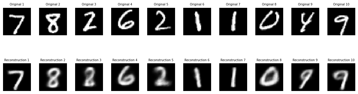
Another helper function to sample from our latent space and generate new images based on random latent vectors. Isnt this amazing for 10 epochs?
# now let us create a function that will sample from our latent space and generate new images based on random latent vectors
def generate_image_from_latent_space(model, device, n_samples=10):
model.eval().to(device) # Set the model to evaluation mode and move to device
# Generate random latent vectors with shape (n_samples, latent_dim)
latent_vectors = torch.randn(n_samples, 3).to(device) # Latent space with 3 dimensions
# Pass the latent vectors through the decoder to generate images
with torch.no_grad():
generated_images = model.decode(latent_vectors)
# Plot the generated images
fig, axes = plt.subplots(1, n_samples, figsize=(15, 4))
for i, ax in enumerate(axes):
ax.imshow(generated_images[i].view(28, 28).cpu().detach().numpy(), cmap='gray')
ax.axis('off')
ax.set_title(f'Sample {i+1}', fontsize=7)
plt.show()
# call the function above
generate_image_from_latent_space(_model, _device, 10)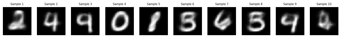
Now time for you to play with the actual model yourself, you can use the sliders and see the magic in realtime!
Use the interactive sliders below to generate samples from the latent 3d vector of your choosing in real time
VAE Image Generator
00
0
Generated Image: